引子
主成分分析(Principal component analysis,PCA)是由Pearson在1901年提出的,后来被Hotelling在1933进行了发展。PCA目的是把多个相关的原始变量降维成少数几个不相关的主成分,其基本原理是原始变量的线性组合。
进行主成分分析的步骤
数据预处理
原始数据矩阵或者相关系数矩阵都可以进行分析,需要注意的几点:
- 原始数据矩阵实际是计算协方差矩阵进行的主成分分析。
- 原始数据矩阵只适用于度量单位相同,或者差别不大时进行分析,如果差别大可以进行Z得分转换。
- 不论是原始数据矩阵还是相关系数矩阵,都不能有缺失值。
确定主成分个数
在计算主成分得分之前,需要先判断主成分个数,通常有四种准则:
- 根据先验经验或者理论知识。
- Kaiser-Harris准则,只保留特征值大于1的主成分。
- Cattell碎石检验,通过绘制特征值与主成分数的图形,只保留在图形变化最大处之上的主成分。
- 平行分析,依据与初始矩阵相同大小的随机数据矩阵来判断要提取的特征值,若基于真实数据的某个特征值大于一组随机数据矩阵相 应的平均特征值,那么该主成分可以保留。
通常需要结合四种准则,综合判断主成分个数。
计算主成分
在R语言中既可以使用base包中的princomp()函数,也可以使用psych包中的principal()函数。
旋转主成分
旋转是一系列将成分载荷阵变得更容易解释的数学方法,它们尽可能地对成分去噪。旋转方法有两种:
- 正交旋转:使选择的成分保持不相关
- 斜交旋转:和让它们变得相关
旋转方法也会依据去噪定义的不同而不同。最流行的正交旋转是方差极大旋转,它试图对载荷阵的列进行去噪,使得每个成分只是由一组有限的变量来解释(即载荷阵每列只有少数几个很大的载荷,其他都是很小的载荷)。
解释结果并计算主成分得分
对结果进行解释,并计算各个主成分的得分,需要注意的是:使用相关系数矩阵进行主成分分析时,无法直接获得主成分得分,只能得到原始变量的主成分系数。
主成分分析的示列
建议在R语言中,使用psych包进行主成分分析。
载入包和数据
示列数据集使用的是psych包中自带的Harman23.cor数据集。Harman23.cor是一个list,需要提取出分析使用的cov数据集.
library(psych)

data(Harman23.cor)
str(Harman23.cor)
List of 3
 $ cov   : num [1:8, 1:8] 1 0.846 0.805 0.859 0.473 0.398 0.301 0.382 0.846 1 ...
  ..- attr(*, "dimnames")=List of 2
  .. ..$ : chr [1:8] "height" "arm.span" "forearm" "lower.leg" ...
  .. ..$ : chr [1:8] "height" "arm.span" "forearm" "lower.leg" ...
 $ center: num [1:8] 0 0 0 0 0 0 0 0
 $ n.obs : num 305
df <- Harman23.cor$cov
str(df)
 num [1:8, 1:8] 1 0.846 0.805 0.859 0.473 0.398 0.301 0.382 0.846 1 ...
 - attr(*, "dimnames")=List of 2
  ..$ : chr [1:8] "height" "arm.span" "forearm" "lower.leg" ...
  ..$ : chr [1:8] "height" "arm.span" "forearm" "lower.leg" ...
判断主成分个数
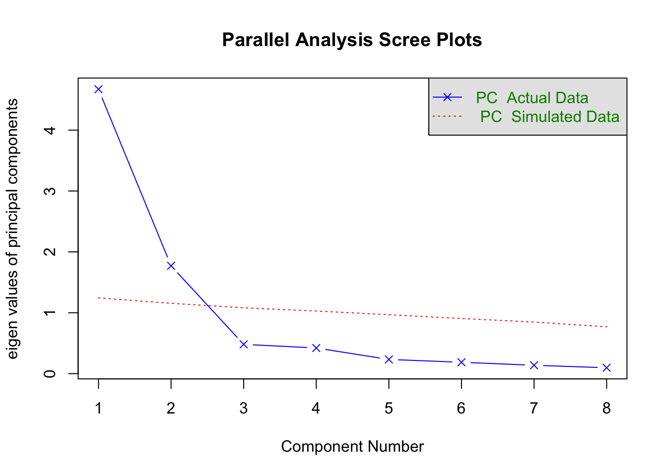
psych包中给出了一个特别有用的函数fa.parallel(),可以很方便的同时给出Kaiser-Harris准则、Cattell碎石检验、平行分析的结果。由上步骤可以看出,df实际为相关系数矩阵,n.obs是指定原始观测数,n.iter是指定平行分析的随机迭代次数,fa是用来指定进行主成分分析,取值有三类(‘fa’,‘pc’,‘both’)。由 图 8.1 看出,特征值大于1,拐点之上,大于随机的特征值,满足以上三个条件,只有前两个主成分,因此主成分个数为2.
fa.parallel(df,
            n.obs = 302,
            n.iter = 100,
            fa = 'pc',
            show.legend = TRUE)
Parallel analysis suggests that the number of factors = NA and the number of components = 2
主成分分析
结果中:
- PC1和PC2既为2个主成分在各个原始变量上的载荷(loading,也就是相关系数),可以看出系数都较高。
- h2为成分公因子方差,用来说明主成分对每个变量的方差解释度,此值越高说明解释力度越大。
- u2栏指成分唯一性——方差,用来说明无法被主成分解释的比例,h2与u2之和为1。
- Proportion Var为每个主成分对整个数据集的解释程度。
- Cumulative Var是Proportion Var的累计和,其值至少应该需大于0.80以上。
可以看出,PC1和PC2在部分变量上都有较高的解释度,不满足各个主成分之间应该正交的条件,需进行旋转。
principal(df,
          nfactors = 2,
          rotate = 'none',
          n.obs = 302,
          scores = TRUE)
Principal Components Analysis
Call: principal(r = df, nfactors = 2, rotate = "none", n.obs = 302,
    scores = TRUE)
Standardized loadings (pattern matrix) based upon correlation matrix
                PC1   PC2   h2    u2 com
height         0.86 -0.37 0.88 0.123 1.4
arm.span       0.84 -0.44 0.90 0.097 1.5
forearm        0.81 -0.46 0.87 0.128 1.6
lower.leg      0.84 -0.40 0.86 0.139 1.4
weight         0.76  0.52 0.85 0.150 1.8
bitro.diameter 0.67  0.53 0.74 0.261 1.9
chest.girth    0.62  0.58 0.72 0.283 2.0
chest.width    0.67  0.42 0.62 0.375 1.7

                       PC1  PC2
SS loadings           4.67 1.77
Proportion Var        0.58 0.22
Cumulative Var        0.58 0.81
Proportion Explained  0.73 0.27
Cumulative Proportion 0.73 1.00

Mean item complexity =  1.7
Test of the hypothesis that 2 components are sufficient.

The root mean square of the residuals (RMSR) is  0.05
 with the empirical chi square  46.77  with prob <  1.1e-05

Fit based upon off diagonal values = 0.99
从结果可以看出,PC1和PC2变成了RC1和RC2,即表示经过旋转了,可以很清楚的看出:旋转后,RC1在前4个变量(height – lower.leg)上具有更高的解释度。RC2在后4个变量(weight – chest.width)上具有更高的解释度,说明两个主成分正交(不相关),同时可以发现,旋转后并不改变Cumulative Var
dfp <- principal(df, nfactors = 2,
                 rotate = 'varimax',
                 n.obs = 302,
                 scores = TRUE)
dfp
Principal Components Analysis
Call: principal(r = df, nfactors = 2, rotate = "varimax", n.obs = 302,
    scores = TRUE)
Standardized loadings (pattern matrix) based upon correlation matrix
                RC1  RC2   h2    u2 com
height         0.90 0.25 0.88 0.123 1.2
arm.span       0.93 0.19 0.90 0.097 1.1
forearm        0.92 0.16 0.87 0.128 1.1
lower.leg      0.90 0.22 0.86 0.139 1.1
weight         0.26 0.88 0.85 0.150 1.2
bitro.diameter 0.19 0.84 0.74 0.261 1.1
chest.girth    0.11 0.84 0.72 0.283 1.0
chest.width    0.26 0.75 0.62 0.375 1.2

                       RC1  RC2
SS loadings           3.52 2.92
Proportion Var        0.44 0.37
Cumulative Var        0.44 0.81
Proportion Explained  0.55 0.45
Cumulative Proportion 0.55 1.00

Mean item complexity =  1.1
Test of the hypothesis that 2 components are sufficient.

The root mean square of the residuals (RMSR) is  0.05
 with the empirical chi square  46.77  with prob <  1.1e-05

Fit based upon off diagonal values = 0.99
计算主成分得分
在principal函数中的scores即是制定是否计算主成分得分的,如果为TRUE,则在dfp中已保存有得分,利用dfp$scores即可以取出得分。但是本示列中使用的是相关系数矩阵,无法计算得分,只能计算得分权重,为:
                       RC1         RC2
height          0.27524417 -0.04748169
arm.span        0.29673051 -0.08005490
forearm         0.29823990 -0.09158460
lower.leg       0.28014088 -0.06027214
weight         -0.06053059  0.33228637
bitro.diameter -0.07752349  0.32477593
chest.girth    -0.10366026  0.33763942
chest.width    -0.03730720  0.27392667